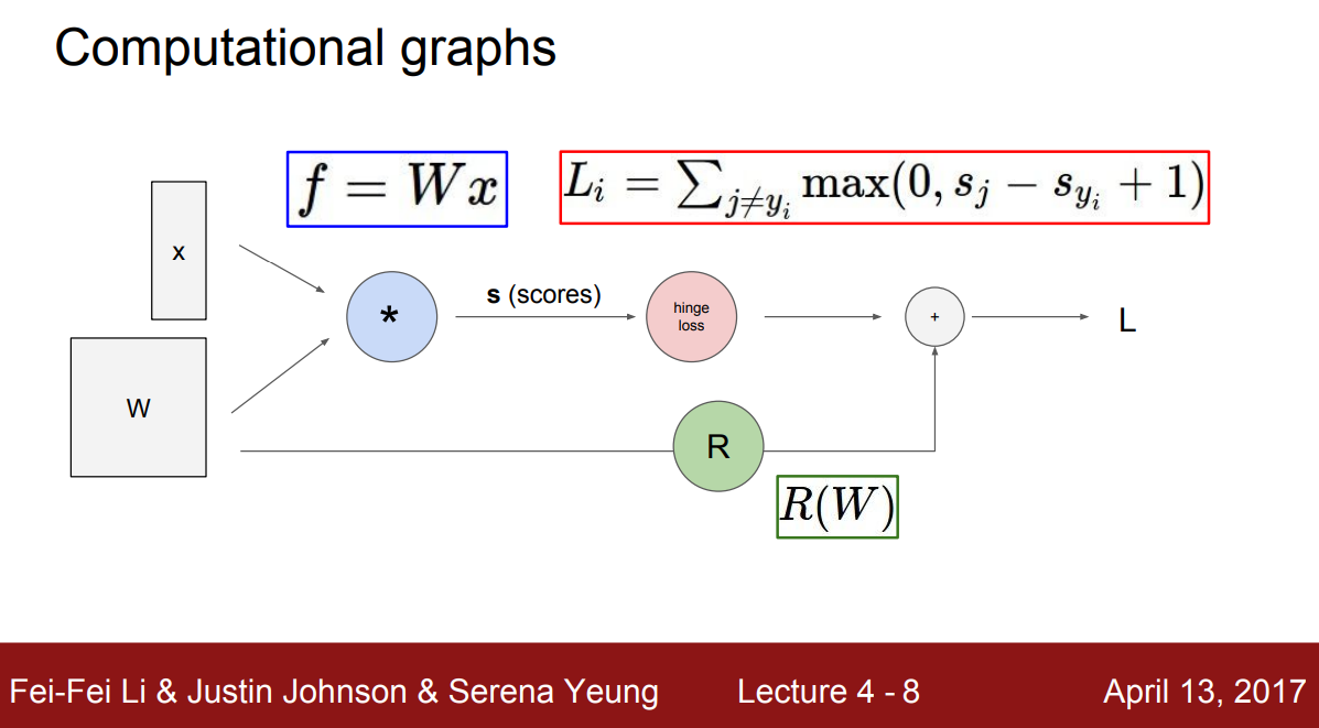
Wikipedia: Backpropagation computes the gradient of a loss function with respect to the weights of the network for a single input–output example. Recursive application of chain-rule along the computational graph to compute the gradients for all input and parameters.
Computational Graph
A computational graph is defined as a directed graph where the nodes correspond to mathematical operations. Computational graphs are a way of expressing and evaluating a mathematical expression.
 source: http://cs231n.stanford.edu/slides/2017/cs231n_2017_lecture4.pdf
Compute the Gradient
- Numerical gradient (use limit rule)
- easy but approximate and slow
- Analytic gradient (manually compute the derivative of a function)
- fast and exact, error-prone (because we might make mistake when computing the gradient manually) in practice: write the analytic gradient and validate it using numerical gradient
Backpropagation in detail
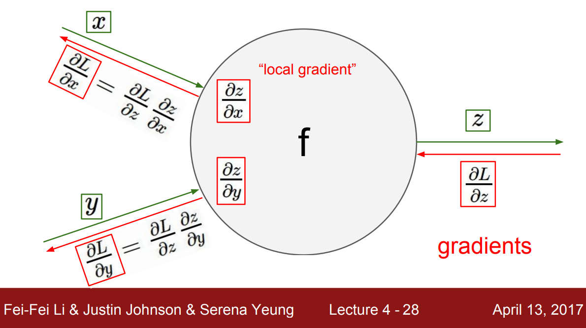
 source: http://cs231n.stanford.edu/slides/2017/cs231n_2017_lecture4.pdf
for each node:
- we start from the end all the way to the beginning and then when we reach each node:
- we have the “upstream gradient” coming back with respect to the immediate output node (in the image above we have the gradient of $L$ in respect of $z$ aka $\delta L/\delta z$)
- we want to find the gradient in respect just before the node (in the example above in respect of $x$ and $y$ or $\delta L/\delta x$ and $\delta L/\delta y$)
- to do that first we calculate the “local gradient” of x in respect to z and y in respect to z
- then we multiply the upstream gradient with the local gradient to get the gradient of x and y in respect to L using the chain rule
- $\delta L/\delta x = \delta L/\delta z \ * \delta z/\delta x$
- $\delta L/\delta y = \delta L/\delta z \ * \delta z/\delta y$
in practice: the implementations maintain a graph structure, where all the nodes implement forward() and backward() API for forward propagation and the backward propagation